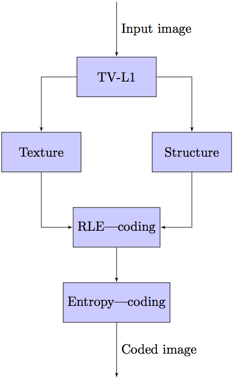
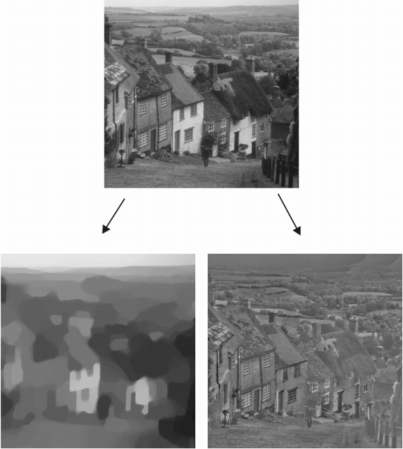
Separate texture and structure processing for imagecompression

Frantc V. A.^a, Makov S. V.^a, Voronin V. V.^a, Marchuk V. I.^a, and Svirin I. S.^b

^aDon State Technical university, Dept, of Radio-Electronics Systems, Gagarina 1, Rostov-on-Don, Russian Federation
^bCJSC Nordavind, Moscov, Russian Federation

ABSTRACT

In the paper we propose approach for lossless image compression. Proposed method is based on separate processing of two image components: structure and texture. In the subsequent step separated components are compressed by standard RLE/LZW coding. We have performed a comparative analysis with existing techniques using standard test images. Our approach have shown promising results.

Keywords - lossless image compression, total-variation regularization, separate image compression

1. INTRODUCTION

At present time the image compression methods suppose to met ever growing requirements. It is related to evolution of imaging systems. It is common for mobile devices to be able to capture Ultra HD video. Captured images should be transferred by communication networks and stored with maximal efficiency. Various kinds of medical devices generate high resolution images that cannot be compressed with lossy techniques because of small changes image can be misinterpreted by a physician. In the same time, plenty of other applications require lossless image compression. Lossless image compression algorithm tends to represent image in such a way that it could be compressed efficiently with standard entropy or dictionary-based information representation techniques to remove all perceptual and statistical redundancy are removed without considerable impact on visual quality.

There is considerable success in this field during past decade. But still, current techniques are far from being universally effective. In the paper we study the possibility of separate image texture and structure lossless compression.

2. PREVIOUS WORK

Lossless image compression have been very active field of research.1 Large amount of data is necessary to represent the digital images so the transmission and storage of such images are time-consuming and infeasible. Hence the information in the images is compressed by extracting only the visible elements. Normally the image compression technique can reduce the storage and transmission costs. During image compression, the size of a graphics file is reduced in bytes without disturbing the quality of the image beyond an acceptable level. Several methods such as Discrete Cosine Transform (DCT), DWT, etc. are used for compressing the images. But, these usually cannot be implemented to be lossless in efficient manner. DCT is employed to compress the color image while the fractal image compression is employed to evade the repetitive compressions of analogous blocks.

Lossy image compression methods that are currently in use are based on Fourier or wavelet transform followed by quantization and entropy coding steps. Recently, proposals have been made to integrate different computer vision techniques into frameworks for image and video coding. These schemes involve texture analysis, segmentation and classification of the signal into ’’texture” and ’’structure” parts. Some methods are designed to code structure with classical approach, but textured regions are synthesized on the decoding side. The employed synthesis methods basically constitute patch-based inpainting of these regions. Therefore, a lot of care has to be taken to perform the segmentation and classification in such a way that visual quality will be the same. Most authors respond to this problem by adding constrains on the classification and synthesis.

In lossless image compression for example, one has to deal with the fact that interesting phenomena occur along curves or sheets, e.g., edges in a two-dimensional image. While wavelets are certainly suitable for dealing

with objects where the interesting phenomena, e.g., singularities, are associated with exceptional points, they are ill-suited for detecting, organizing, or providing a compact representation of intermediate dimensional structures. Given the significance of such intermediate dimensional phenomena, there has been a vigorous research effort to provide better adapted alternatives by combining ideas from geometry with ideas from traditional multiscale analysis.2

In its original formulation, presented by Perona and Malik2 the space-variant filter is in fact isotropic but depends on the image content such that it approximates an impulse function close to edges and other structures that should be preserved in the image over the different levels of the resulting scale space. This formulation was referred to as anisotropic diffusion by Perona and Malik even though the locally adapted filter is isotropic, but it has also been referred to as inhomogeneous and nonlinear diffusion3 or Perona-Malik diffusion4 by other authors. A more general formulation allows the locally adapted filter to be truly anisotropic close to linear structures such as edges or lines: it has an orientation given by the structure such that it is elongated along the structure and narrow across. Such methods are referred to as shape-adapted smoothing5 or coherence enhancing diffusion. As a consequence, the resulting images preserve linear structures while at the same time smoothing is made along these structures. Both these cases can be described by a generalization of the usual diffusion equation where the diffusion coefficient, instead of being a constant scalar, is a function of image position and assumes a matrix (or tensor) value (see structure tensor). Lossy image compression methods that are currently in use are based on Fourier or wavelet transfrom followed by quantization and entropy coding steps. Recently, proposals have been made to integrate different computer vision techniques into frameworks for image and video coding.6 These schemes involve texture analysis, segmentation and classification of the signal into ’’texture” and ’’structure” parts. Authors of7 code structure with classical approach, but textured regions are synthesized on the decoding side. The employed synthesis methods8 basically constitute patch-based compression of this regions. Therefore, a lot of care has to be taken to perform the segmentation and classification in such a way that visual quality will be the same. Most authors respond to this problem by adding constrains on the classification and synthesis. In the paper9 analogous blocks are found by using the Euclidean distance measure. Here, the given image is encoded by means of Huffman encoding technique. The implementation result shows the effectiveness of the proposed scheme in compressing the color image. Also, a comparative analysis is performed to prove that our system is competent to compress the images in terms of Peak Signal to Noise Ratio (PSNR), Structural Similarity Index (SSIM) and Universal Image Quality Index (UIQI) measurements. The paper10 describes some recent developments that have taken place in context-based predictive coding, in response to the JPEG/JBIG committees recent call for proposals for a new international standard on lossless compression of continuous-tone images. We describe the different prediction techniques proposed and a performance comparison is given. We describe the notion of context-based bias cancellation, which represents one of the key ideas that was proposed and incorporated in the final standard. We also describe the different error modelling and entropy coding techniques that were proposed for encoding prediction errors, the most important development here being an ingeniously simple and effective technique for adaptive GolombRice coding. We conclude with a short discussion on avenues for future research.

Although the resulting family of images can be described as a combination between the original image and space-variant filters, the locally adapted filter and its combination with the image do not have to be realized in practice and there is a place for future investigation.

3. SEPARATE TEXTURE AND STRUCTURE CODING USING TV-L1

Proposed way of image compression is shown on figure 1. First image is separated on two components: ’’structure” and ’’texture”. To estimate the image structure we apply total variation anisotropic smoothing.14 We use algorithm of total variation minimisation proposed by Antonin Chambolle in6 . Then we compute image texture as the difference between the source image and image structure. So the sum of structure and texture components will be equal to original image on figure 2.

An image can be modelled as a function u : Ω → R where Ω R 2. In the discrete settings 1, 2, . . . , n × 1, 2, . . . , m → R.

The general idea in order to decompose an image into s + t is given by Meyer’s models:11

Figure 1. Blockscheme

here F₁, F₂ ≥ 0, X₁, X₂ are functional spaces or distributions such that X1 = {s : F₁(s) < ∞} and X₂ = {t : F₂(t) < ∞} and X₂ = {v : F₂(v) < ∞} The constant λ > 0 is a tuning parameter. Many problems in imaging can be represented by this model withan appropriate choice of F₁ and F₂. In our particular case, we are looking for two spaces X₁ and X₂ , and two corresponding functionals F₁ and F₂, such that if s is structure and t is texture, we have F₁(s) << F₂(s) and F₁(t) >> F₂(t). Here texture component must be penalized by F₁, and structure component should be penalized by F₂. Total variation minimization is a convex variational method that plays an important role in imaging as it allows for sharp discontinuities in the solution. However, it is known to be difficult to minimize due to the non-smoothness of the objective function. A good choice for F₁ is the total variation of u, that tends to involve constant regions and permits sharp edges, that are necessary for the structure part. It remains to discuss what space X₂ would model the textural part. TV model is:

(2)

here

(3)

denotes the total variation of u in Ω, also denoted by . The component u belongs to the space of functions with bounded variation .

The space of functions with bounded variation penalizes fast changes of the image (such as noise or texture), but allows for piecewise-smooth functions, made of homogeneous regions with smooth contrasted boundaries. Since almost all level lines (or isolines) of a BV function have finite length, the BV space is considered adequate to model images containing shapes. We have chosen6 method for solving the TV − L1 problem. This method is based on smoothing of the TV

Image

Structure Texture

term:

(4)

Different optimization techniques based on total variation-based regularisation was applied in the field of image processing. Let’s introduce notations used in the rest of the paper. In the continuous setting, a grey scale image can be modelled as a function u : Ω → R. Here ω ⊂ R 2 is usually a rectangle and u(x) is the intensity of the grey level at the point x. In the discrete setting an image is a function u : {1, 2, . . . , n} × {1, 2, . . . , m} → R with m × n - resolution of image. To tackle the task of image compression we first separate image to two components u = s + t, where s denotes structural part of image and t is textural information.

Let Ω ⊂ R 2 to denote a subset of the plane and I(·, t) : Ω → R be a family of gray scale images, then anisotropic diffusion is defined as = div (c(x, y, t)∇I) = ∇c ·∇I +c(x, y, t)∆I where ∆ denotes the Laplacian, ∇ denotes the gradient, div(. . .) is the divergence operator and c(x, y, t) is the diffusion coefficient. c(x, y, t) controls the rate of diffusion and is usually chosen as a function of the image gradient so as to preserve edges in the image. Pietro Perona and Jitendra Malik pioneered the idea of anisotropic diffusion in 1990 and proposed two functions for the diffusion coefficient:

(5)

and

(6)

the constant K controls the sensitivity to edges and is usually chosen experimentally or as a function of the noise in the image. Let M denote the manifold of smooth images, then the diffusion equations presented above can be interpreted as the gradient descent equations for the minimization of the energy functional E : M → R defined by

 where g : R —> R is a real-valued function which we will see is intimately related to the diffusion coefficient. Then for any compactly supported infinitely differentiable test function h , we have:

(7)

(8)

(9)

where the last line follow from multidimensional integration by parts. Letting ∇E₁ denote the gradient of E with respect to the L² (Ω, R) inner product evaluated at I, this gives

Therefore, the gradient descent equations on the functional E are given by Thus by letting c = g’ we obtain the anisotropic diffusion equations.

Modified Perona-Malik model⁵ (that is also known as regularization of P-M equation) will be discussed in this section. In this approach, the unknown is convolved with a Gaussian inside the non-linearity to obtain the modified Perona-Malik equation:

(10)

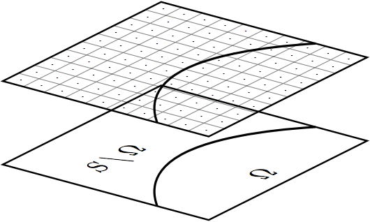
The well-posedness of the equation can be achieved by regularization but it also introduce blurring effect, which is the main drawback of regularization. A prior knowledge of noise level is required as the choice of regularization parameter depends on it.

Then the both components are encoded by RLE and LZW. Image splitting is schematically represented on figure 3. Here Ω is textured region and S is the whole image.

Figure 3. Image separation

In numerical and functional analysis, a discrete wavelet transform (DWT) is any wavelet transform for which the wavelets are discretely sampled. As with other wavelet transforms, a key advantage it has over Fourier transforms is temporal resolution: it captures both frequency and location information (location in time). Compression process is very similar to that of a conventional coder such as JPEG. However, the functionality is very different. In a conventional coder, since the quantization result is losslessly encoded, the quantization process determines the allowable distortion of the transform coefficients. The quantized coefficients are lossy encoded through an embedded coder, thus additional distortion can be introduced in the entropy coding steps. Thus, the main functionality of the quantization module is to map the coefficients from floating representation into integer so that they can be more efficiently processed by the entropy coding module. The image coding quality is not determined by the quantization step size 5 but by the subsequent bit stream assembler.

4. COMPARISON WITH EXISTING APPROACHES

A high level view of the encoding algorithm is shown here:

1. Initialize the dictionary to contain all strings of length one.
2. Find the longest string W in the dictionary that matches the current input.
3. Emit the dictionary index for W to output and remove W from the input.
4. Add W followed by the next symbol in the input to the dictionary.
5. Go to Step 2

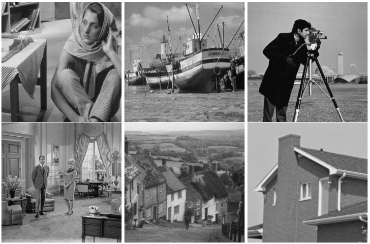
A dictionary is initialized to contain the single-character strings corresponding to all the possible input characters (and nothing else except the clear and stop codes if they’re being used). The algorithm works by scanning through the input string for successively longer sub-strings until it finds one that is not in the dictionary. When such a string is found, the index for the string without the last character (i.e., the longest substring that is in the dictionary) is retrieved from the dictionary and sent to output, and the new string (including the last character) is added to the dictionary with the next available code. The last input character is then used as the next starting point to scan for sub-strings.

For evaluation purposes we use image dataset of 6 natural images presented at Figure 4.

We compare our technique to two different ones. The first is based on Haar transform, and the second one on Gaussian smoothing.

4.1 Haar transform for image separation

For this method source image is decomposed to high and low frequency components. Standard DB9 wavelet transform is sufficient to code structural information. So we code textural information with standard JPEG2000 compression scheme. To apply a wavelet transform to an image we need to use a 2D version. In this case it is common to apply the wavelet transform separatelly in horizontal and vertical directions. This approach is called the separable 2D wavelet transform. It is possible to design a non separable 2D wavelet, but this is generally increases computational complexity with little additional coding gain. A sample one scale separable 2D wavelet transform. It is possible to design a non separable 2D wavelet, but this generally increases computational complexity with little additional coding gain.

The 2D data array representing the image is first filtered in the horizontal direction, which results in two sub-bands: a horizontal low-pass and a horizontal high-pass sub-band. These sub-bands are then passed through a vertical wavelet filter. The image is thus decomposed into four sub-bands: LL (low-pass horizontal and vertical filter), LH(low-pass vertical and high-pass horizontal filter), HL (high-pass vertical and low- pass horizontal filter) and HH (high-pass horizontal and vertical filter). Since the wavelet transform is linear, we may switch the order of the horizontal and vertical filters yet still reach the same effect. By further decomposing sub-band LL with another 2D wavelet (and iterating this procedure), we derive a multiscale dyadic wavelet pyramid.

Figure 4. Test images

The DWT of a signal x is calculated by passing it through a series of filters. First the samples are passed through a low pass filter with impulse response g resulting in a convolution of the two:

(11)

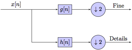
The signal is also decomposed simultaneously using a high-pass filter h. The outputs giving the detail coefficients (from the high-pass filter) and approximation coefficients (form the low-pass). It is important that the two filters are related to each other (Figure 5).

Figure 5. Control system

However, since half the frequencies of the signal have now been removed, half the samples can be discarded according to Nyquist’s rule. The filter outputs are then sub sampled by 2. In the next two formulas, the notation is the opposite: g-denotes high pass and h−low pass as is Mallat’s and the common notation:

(12)

(13)

This decomposition has halved the time resolution since only half of each filter output characterises the signal. However, each output has half the frequency band of the input so the frequency resolution has been doubled. With the sub sampling operator ↓.

(14)

(15)

However computing a complete convolution x*g with subsequent down sampling would waste computation time. The Lifting scheme is an optimization where these two computations are interleaved.

4.2 Gaussian smoothing for image decomposition

In mathematics, a Gaussian function, often simply referred to as a Gaussian, is a function of the form:

(16)

for arbitrary real constants a, b and c. The graph of a Gaussian is a characteristic symmetric ’’bell curve” shape. The parameter a is the height of the curve’s peak, b is the position of the center of the peak and c (the standard deviation, sometimes called the Gaussian RMS width). We use Gaussian smoothing to separate image to two components: high frequency and low frequency one.

4.3 Experimental results

Experimental results are presented in table 1 (less is better). Numbers represent a ratio of uncompressed image data and data preprocessed by given approach and then compressed with RLE+LZW.

Table 1. Table 1 — Compression rate

We had run our method on images from Inria Holydays dataset18 which contains 1491 images in total. This dataset includes large variety of scene types and thus is suitable for benchmarking of compression method. On this dataset we were able to determine that our method of image decomposition is superior to others in 71% of the time. Average compression rate for our method is 0.21. Gaussian and Haar decomposition got 0.24 and 0.26 respectively. Our approach usually perform better for images with number of highly stochastic textures occupying relatively big regions.

As you can see our approach is superiour to Gaussian and Haar-based splitting. Particular compression ration is related to amount and spatial allocation of different textural and structural components.

5. CONCLUSION

The paper presents a lossless image compression technique based on image texture and structure separation. To estimate the image structure we applied the total variation anisotropic smoothing. Then we computed image texture as the difference between the source image and image structure. The both components are encoded by RLE and LZW. Experimental comparisons to state-of-the-art video compression methods demonstrate the effectiveness of the proposed approach.

6. ACKNOWLEGEMENT

This work was supported by Russian Ministry of Education and Science in frame of the Federal Program ” Research and development on priority directions of scientific-technological complex of Russian Federation in 2014- 2020” (contract #14.576.21.0080 (RFMEFI57614X0080)).

REFERENCES

1. Rawat, Chandan, and Sukadev Meher. ” A Hybrid Image Compression Scheme Using DCT and Fractal Image Compression.” Int. Arab J. Inf. Technol. 10.6 (2013): 553-562.
2. Candes, Emmanuel, et al. ’’Fast discrete curvelet transforms.”Multiscale Modeling and Simulation 5.3 (2006): 861-899.
3. Le Guen, Vincent. ”Cartoon+ Texture Image Decomposition by the TV-L1 Model.” Image Processing On Line 4 (2014): 204-219.
4. Marcellin M. W. et al. An overview of JPEG-2000 //Data Compression Conference, 2000. Proceedings. DCC 2000 IEEE, 2000. . 523-541.
5. Papafitsoros K., Schoenlieb С. B., Sengul B. Combined first and second order total variation inpainting using split Bregman //Image Processing On Line. 2013. . 2013. . 112-136.
6. Chambolle, Antonin. ”An algorithm for total variation minimization and applications.” Journal of Mathematical imaging and vision 20.1-2 (2004): 89-97.
7. P. Saisan, G. Doretto, Ying Nian Wu, and S. Soatto. Dynamic texture recognition. In Proceedings of the Conference on Computer Vision and Pattern Recognition, volume 2, pages 5863, Kauai, Hawaii, December 2001.
8. Weinberger, Marcelo J., Gadiel Seroussi, and Guillermo Sapiro. ’’The LOCO-I lossless image compression algorithm: principles and standardization into JPEG-LS.” Image Processing, IEEE Transactions on 9.8 (2000): 1309-1324.
9. Weinberger, Marcelo J., Gadiel Seroussi, and Guillermo Sapiro. ’’LOCO-I: A low complexity, context-based, lossless image compression algorithm.” Data Compression Conference, 1996. DCC’96. Proceedings. IEEE, 1996.
10. Calderbank, A., et al. ’’Lossless image compression using integer to integer wavelet transforms.” icip. IEEE,
11. Howard, Paul G., and Jeffrey Scott Vitter. ’’Fast and efficient lossless image compression.” (1993).
12. Reichel, Julien, et al. ’’Integer wavelet transform for embedded lossy to lossless image compression.” Image Processing, IEEE Transactions on 10.3 (2001): 383-392.
13. Maniccam, S. S., and Nikolaos G. Bourbakis. ’’Lossless image compression and encryption using SCAN.” Pattern Recognition 34.6 (2001): 1229-1245.
14. Boulgouris, Nikolaos V., Dimitrios Tzovaras, and Michael Gerassimos Strintzis. ’’Lossless image compression based on optimal prediction, adaptive lifting, and conditional arithmetic coding.” Image Processing, IEEE Transactions on 10.1 (2001): 1-14.
15. Memon, Nasir, and Xiaolin Wu. ’’Recent developments in context-based predictive techniques for lossless image compression.” The Computer Journal 40.2 and 3 (1997): 127-136.
16. Sahni, S., et al. ’’Lossless Image Compression.” Encyclopedia of Optical Engineering: Las-Pho, pages 1025- 2048 2 (2003): 1177.
17. Memon, Nasir D., and Khalid Sayood. ’’Lossless image compression: A comparative study.” IS&T/SPIE’s Symposium on Electronic Imaging: Science & Technology. International Society for Optics and Photonics, 1995.
18. Jegou, Herve, Matthijs Douze, and Cordelia Schmid. ’’Hamming embedding and weak geometric consistency for large scale image search.” Computer VisionECCV 2008. Springer Berlin Heidelberg, 2008. 304-317.